More details here on the exact approaches we used to scan the entire common crawl, categorise etc.
Big Data Technology
For running jobs across the common crawl we implemented several Hadoop MapReduce jobs using the MRJob python interface. Depending on the specific step, we provisioned a variable number of nodes running on IBM softlayer (www.softlayer.com) servers. The most computationally intensive step in the process takes 300-500 CPU-hours to process depending on the size of the common crawl snapshot.
We stream each common crawl snapshot directly from S3 during each MapReduce job. Approaching the problem this way allows us to throttle the cost of our infrastructure down to zero when not in use. Beyond a certain point, increases in CPU count per node will trigger network bottlnecking. Clusters need a minimum number of nodes to process the data in a reasonable amount of time. 20+ machines equipped with 100MBPS connections are sufficient to complete most jobs within 2 hours.
Decompressing each data file was a huge target for performance improvements. Since the python gzip module is quite slow, we elected to stream gzip content to MapReduce using the native Linux gunzip library. Creating a streamed subprocess call resulted in 10x reduction in running times for the decompression process.
Machine Learning Technology
We used the toolkit scikit-learn to do machine learning to classify businesses. We have trained two distinct models for data set annotation which have different performance and uses. Our first model is able to determine if a domain is a business domain with moderate accuracy, precision and recall. Our second model attempts to determine in one pass if a domain is specifically a Berkeley-area business, and works with very high precision but lower recall.
Our final model is a stacked ensemble which combines intermediate probabilities from different pieces of a webpage into a final prediction as to if a page is a business page. Our first classifier runs TF-IDF over the title of a page, which is combined with TF-IDF of the content of a page using logistic regression. We then aggregate the probabilities for each page being part of a business domain into a final probability using XXX.
Mapping Technology
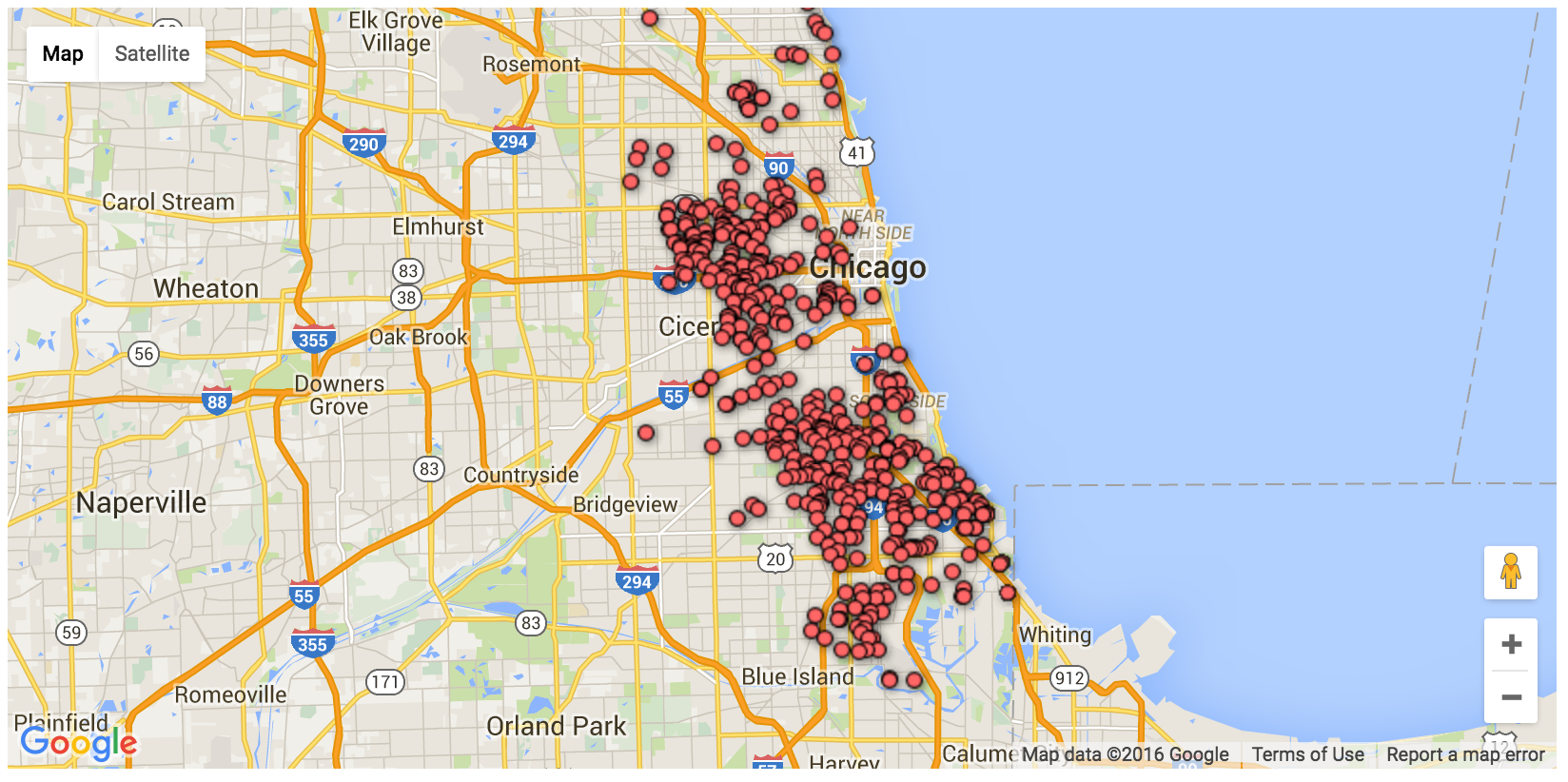
Google Fusion Tables
As mentioned Google Fusion Tables + Google Maps API were used in order to geocode and visualize XXX data points simultaneously for our map visualisation.
TODO: Insert code snippet of ours
An example of provided by Google:
function initMap() {
  var map = new google.maps.Map(document.getElementById('map'), {
    center: {lat: 41.850033, lng: -87.6500523},
    zoom: 11
  });

  var layer = new google.maps.FusionTablesLayer({
    query: {
      select: '\'Geocodable address\'',
      from: '1mZ53Z70NsChnBMm-qEYmSDOvLXgrreLTkQUvvg'
    }
  });
  layer.setMap(map);
}
Limitations of Fusion tables + maps
A note and excerpt on the limitation of using Fusion Tables with Google maps:
Google Maps + Fusion Table Limits
You can use the Google Maps JavaScript API to add up to five Fusion Tables layers to a map, one of which can be styled with up to five styling rules.
In addition:
- Only the first 100,000 rows of data in a table are mapped or included in query results.
- Queries with spatial predicates only return data from within this first 100,000 rows. Therefore, if you apply a filter to a very large table and the filter matches data in rows after the first 100K, these rows are not displayed.